[Electrostatic Headphone Measurements]

Have you had a chance to look at the data with higher resolution I made? I'm wondering if the setting are really doing something in terms of resolution.

I processed the files now and as expected there's little difference. I did not yet check the manual but I think it has to do with the randomness of the MLS sequence but it doesn't actually change the recording settings. e.g. there's still only 3ms of data and the apparent sample rate remains 170kHz something.

[Electrostatic Headphone Measurements]

Have you had a chance to look at the data with higher resolution I made? I'm wondering if the setting are really doing something in terms of resolution.

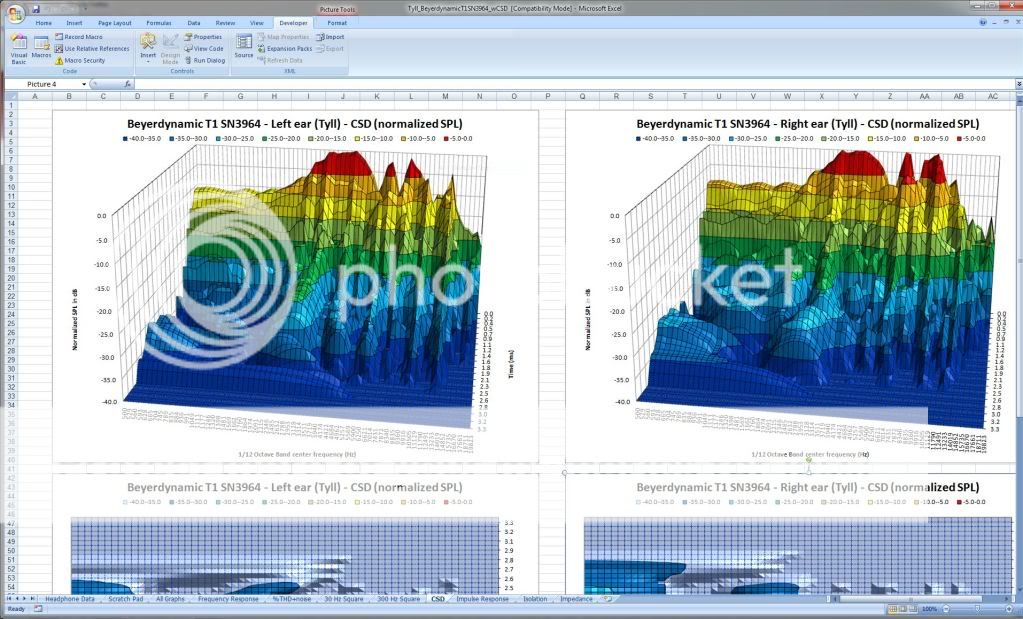
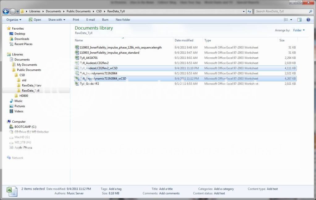
I haven't processed the data but will check later. Meanwhile, per your last PM, I changed the batch routine to also copy the graphs to the original data (new CSD sheet after square wave graphs, graphs pasted as enhanced metafile). It saves the data file as new name with _wCSD suffix just to be safe (file grows from 2MB to 4MB due to the 4 additional graphs).

Illustration:

[Electrostatic Headphone Measurements]

I don't mind chipping in for shipping fees. Actually, people sending your equipment to Tyll, you're paying for shipping one way, which gets pretty expensive for something like a BHSE no??

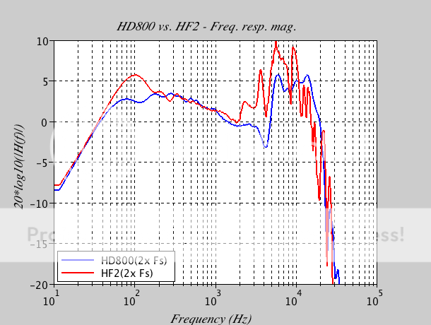
Tyll: I reprocessed Purrin's data with the same Excel template in order to compare your and his measurement of the HF2.

The resemblance is pretty weak which could be due to:

• a blunder in my processing (I get similar results to Purrin's CSD + my FFT at t=0 matches your original spreadsheet result though)
  
• the effect of his measurement method (not traditional dummy head)
  
• some issue with your original data (I don't understand why it shows up as 170kHz sample when your settings show it was actually sampled at 130kHz)
  
• a combination of all the above!!
  

[Electrostatic Headphone Measurements]

That's dedication, many thanks for sending your gear! And more importantly, all the best to your family.

I sent him my OII's with my BHSE. I believe mine are MK1. Well, box says 007A, but the cans are brown leather/cable and champagne housing. Tyll will be able to compare them both side-by-side,

It will be VERY interesting to see how wide the gap is between the two.

[Electrostatic Headphone Measurements]

Had only a very brief look but did not see much difference between your 2 files. I'll have a go at the manual.

Meanwhile, how about changing the settings in the "sweep >>Data3 >" window?

For instance: stop=6ms, Steps=2047.

Or, if you need to specify the time step rather than number of steps, that would be 0.006/2047=2.92969E-06

So I did another test with the longer MLS word (128K) and the next highest sampling rate:

Speadsheet with data for this test is here.

THis shit is pretty complicated, so I figure you might need to look at the manual . Chapter 13 is about MLS and the impulse response etc.

Alrighty, I'm listening for what to do next.

[Electrostatic Headphone Measurements]

Edit: updated graphs, correct a problem with the time scale...

Tyll, I will have a look at your new data and settings. Meanwhile, I could remove the issue (lack of data points) with the current data by automatically zero padding up to 2048 samples and doing the FFTs on that "augmented" data. It does not imagine some new decay beyond 3ms but the low frequency results (below 2kHz) are smoother...

[Electrostatic Headphone Measurements]

Edit: error in CSD graphs, deleted

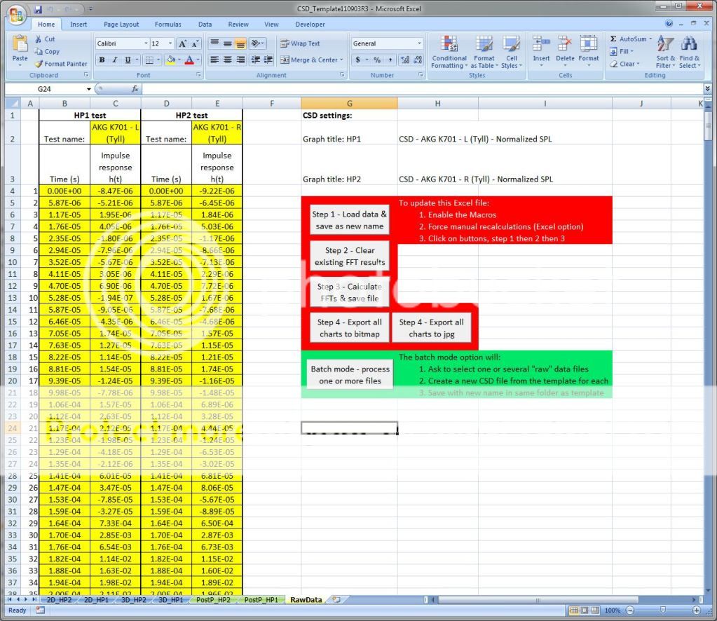
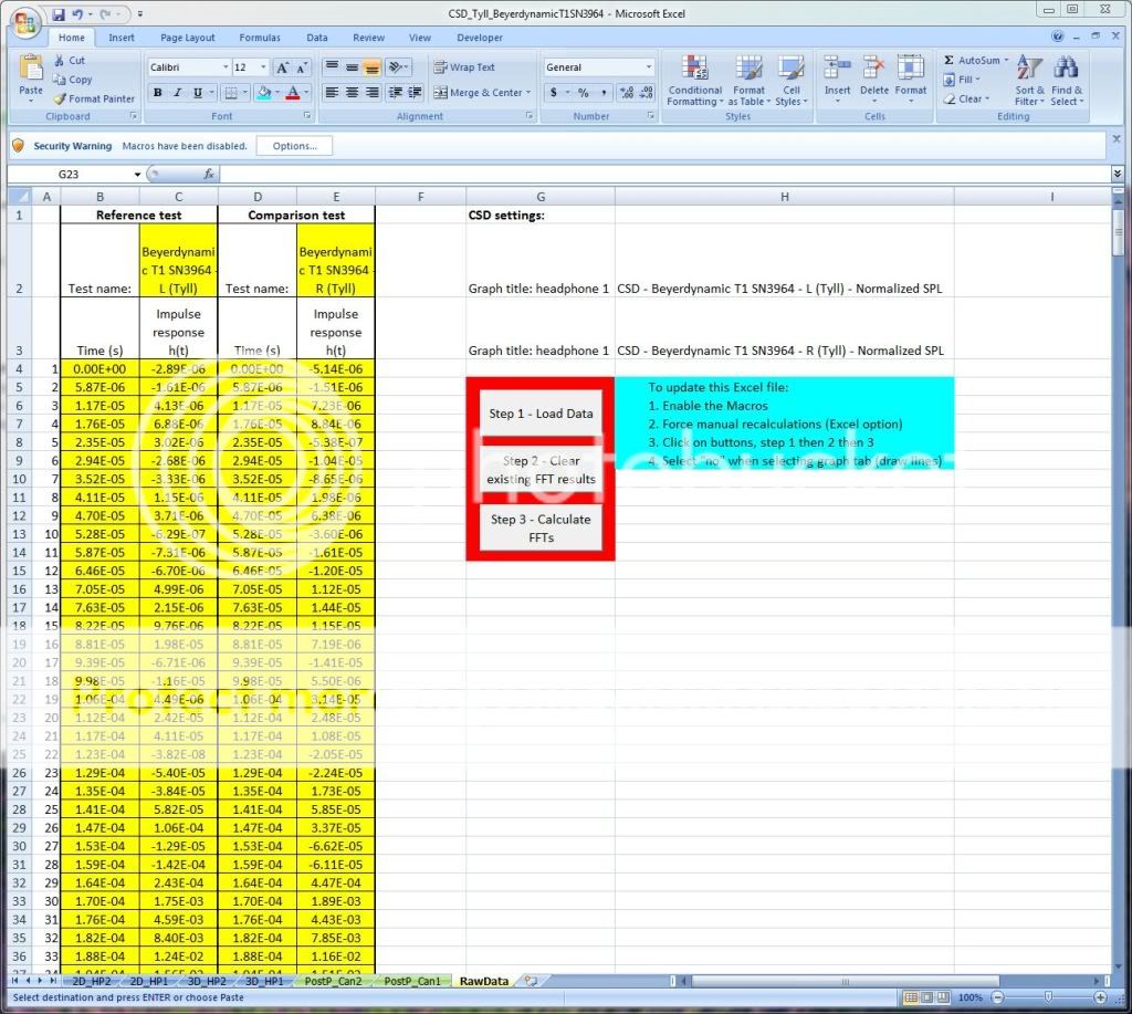
I think I now have a workflow which makes this Excel template usable:

• Can now export all charts automatically to bitmap (4MB file size per chart) or jpg (225kB file size per chart) format
  
• Can now automatically process one or more selected files (in the standard Excel file format you provided us with Tyll)
  

Some example:

[Electrostatic Headphone Measurements]

I am less convinced but really want an explanation or executive summary of this graphy shit.

Simply said, the sharper (frequency) and deeper (decay time) the ridges, the more likely you are to hear these as strong colorations.

[Electrostatic Headphone Measurements]

As an English major, I don't really understand any of this ostentatious sciencing and mathiness. But I am convinced that you gentlemen are doing God's work!

Thanks, you can just enjoy the colors . On my way to add a button to automatically process all the raw data files in the folder, this will really become a "single push button" operation to digest Tyll's 100+ headphones data!

[Electrostatic Headphone Measurements]

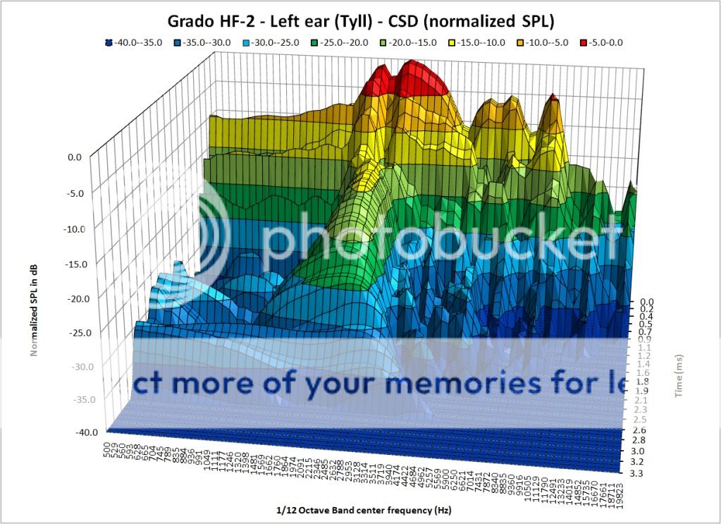
Those look nice. Is there a reason the graphs start at 500 Hz that I missed?

One reason is that most bands don't have any results (the resolution of the original data is not sufficient). Another is that there's very little going on below 1kHz for all the headphones I have seen to date. For instance acoustic resonances in the earcup can't really occur below 2kHz because of the size.

For the electrostatic headphones, as mentionned, we may say a lot of resonances from the thin tensioned diaphragm, but I am not sure where it starts. I'd guess pretty low frequency to prevent too much bass roll off.

In any case, it would be good for Tyll to increase the size of his recordings so that we can look at it from lower frequencies and can see it decay fully naturally.

[Electrostatic Headphone Measurements]

Edit: error in graphs, deleted

Some good news:

1. I can now automatically load the data off Tyll's spreadsheet (using the columns AK and AL as well as cell B2 in the headphone data sheet) to generate the CSD file (3.5MB per headphone, contains both L & R channels).

2. It will be straightforward to create a batch to process you 100+ files Tyll (will generate a new Excel file with CSD_ prefix or the like)

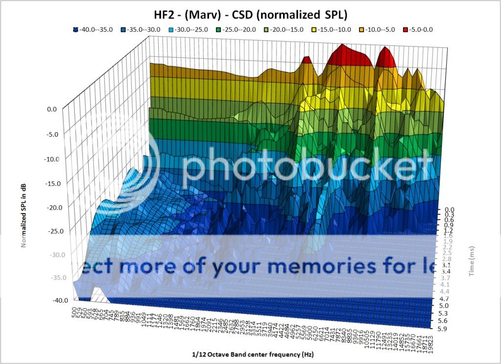
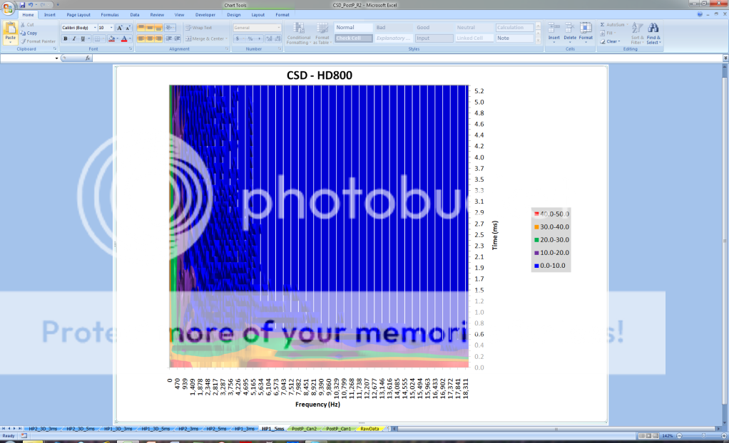
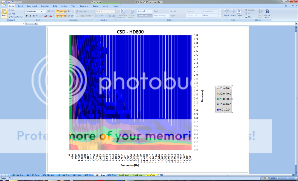
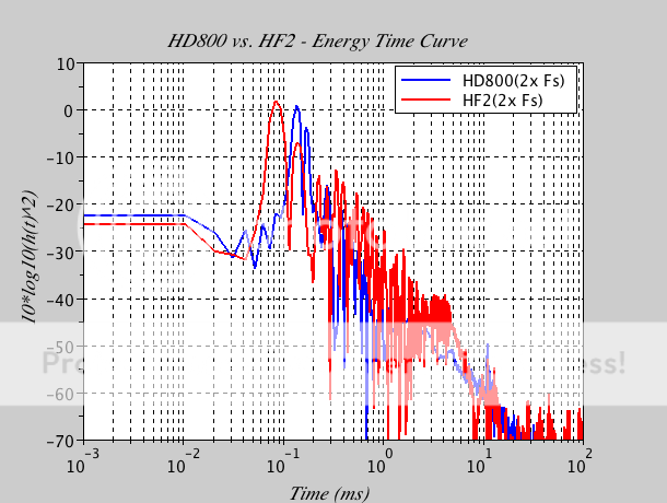
Here are the results from the data you provided Tyll. I did not spend much time on verifying the validity but the t=0 curve seems to match your FRF graph and the CSD seems along the same line as Purrin's results:

[Electrostatic Headphone Measurements]

Tyll, the pleasure is mine, you have and are still investing so much of your time for this hobby of ours, I am glad to help in any way I can.

Couldn't get back to the data you posted, probably better to have some understanding of your current data acquisition system anyway and figure out how to best deal with it after. Just in regards to the lack of data in some bands, we can easily zero pad the existing impulse response and make it artificially longer (3x longer should do). That doesn't fix the potential issue with artificial decay (damping) of the exponential window though, so it would be great if you can find out a bit more about any type of "anti-aliasing" windowing being applied during the FRF estimation.

cheers,

arnaud

[Electrostatic Headphone Measurements]

Sounds like an exponential window was used in the recording to make sure the impulse response fully decayed within the 3ms recording period. I hope this isn't the case as it'll mean the raw data may not be faithfully usable for csd processing...

[Electrostatic Headphone Measurements]

THIS IS STILL NOT RIGHT - MY FR SCALE IS OFF! ASSUMING A WRONG SAMPLE RATE.

You've rushed things a bit Purrin it seems . Sample rate is about 171kHz (1/(t(2)-t(1))). One issue I have is that with only 512 samples of raw data, the frequency resolution of the FFT is too coarse to generate a 1/12OB plot (some bands don't have data inside). Might have to do a composite graph (1/3OB until 1kHz, 1/12OB above that). More tonight...

[Electrostatic Headphone Measurements]

Okay, all you math geeks out there, here's a few spreadsheets to play with.

http://www.innerfide...ges/AKGK701.xls

http://www.innerfide...ezeLCD2Rev2.xls

http://www.innerfide...micT1SN3964.xls

http://www.innerfide...es/GradoHF2.xls

Love to see if the results are similar.

Hi Tyll, is all your data recorded at the same sample rate (170kHz something) and duration (512 samples)?

[Electrostatic Headphone Measurements]

I have a strange feeling we're entering a pissing contest on who's got the prettier graph . Nevertheless, I took note of the Torpedo's comment and created yet another version of the post-processing sheet. How about that?

Only worry is that I feel like the HF2 is giving me the finger for showing it naked in one of the graphs. The old (Josepth?) Grado is clearly more behaved

PS: Tyll, eagerly waiting for your data, let's skype on my sat. early morning if possible!

[Electrostatic Headphone Measurements]

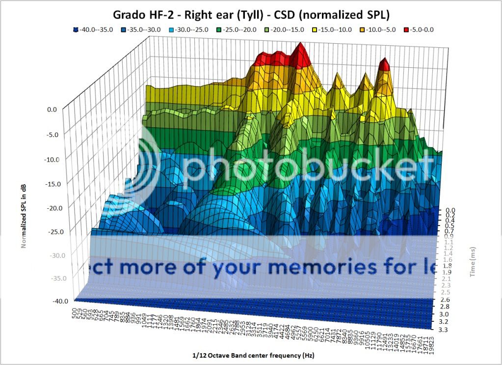
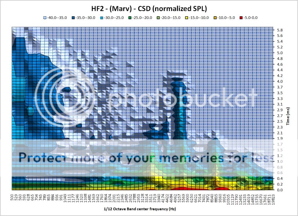
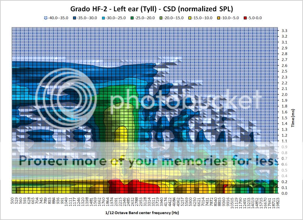
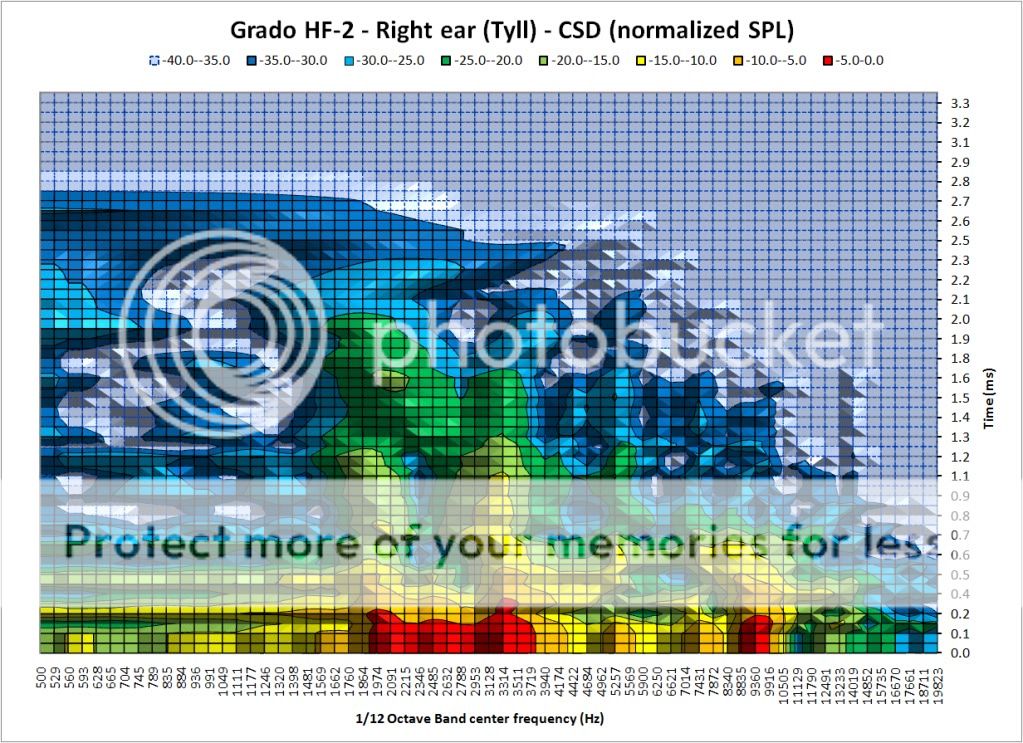
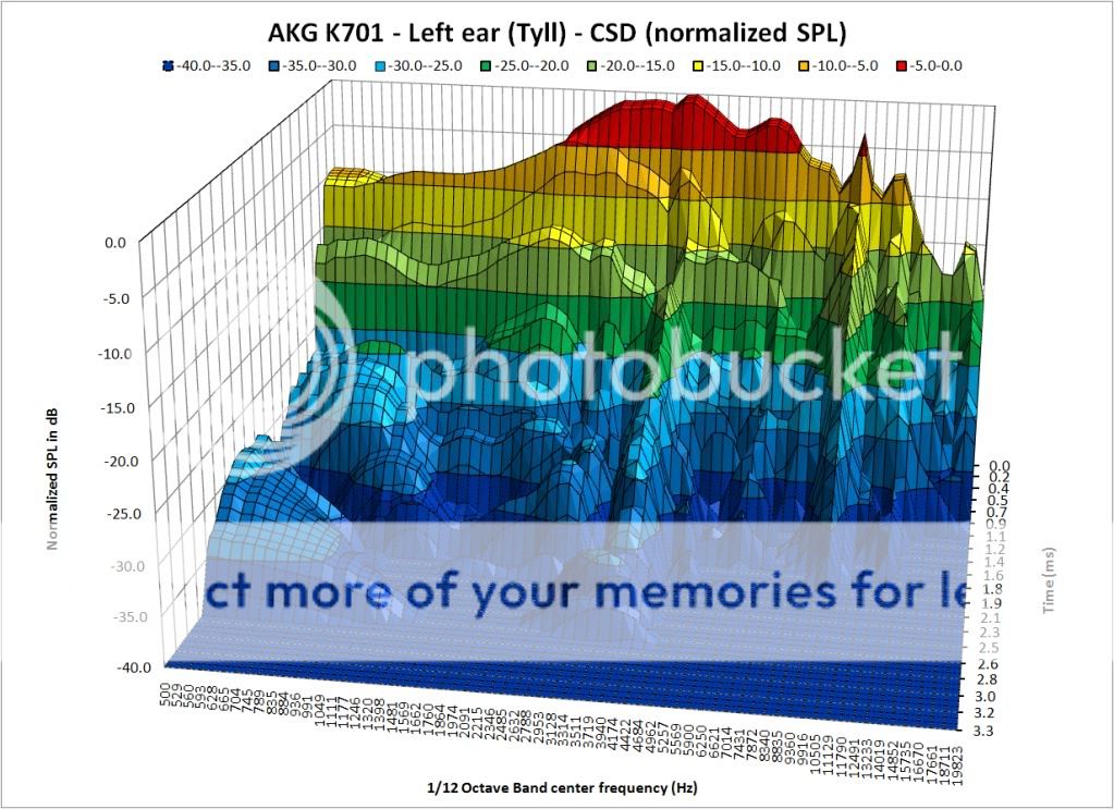
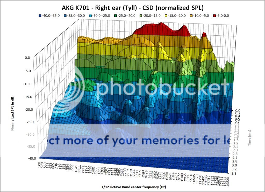
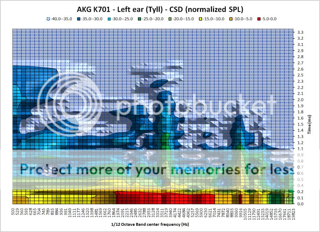
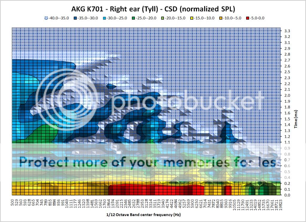
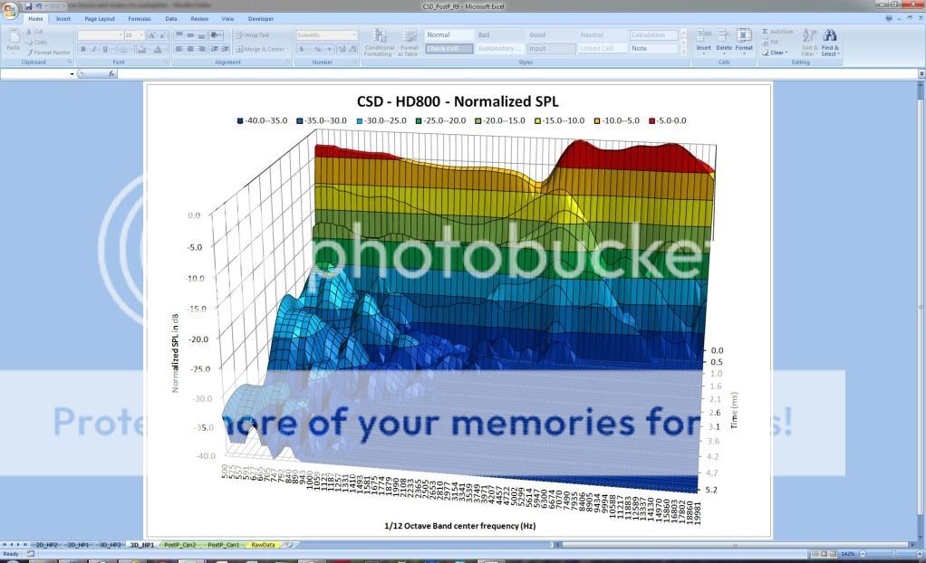
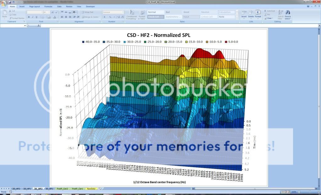
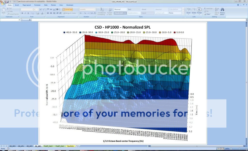
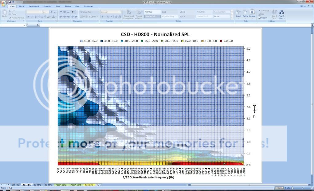
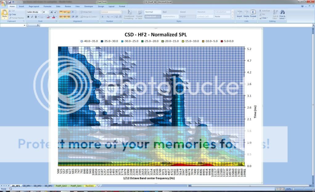
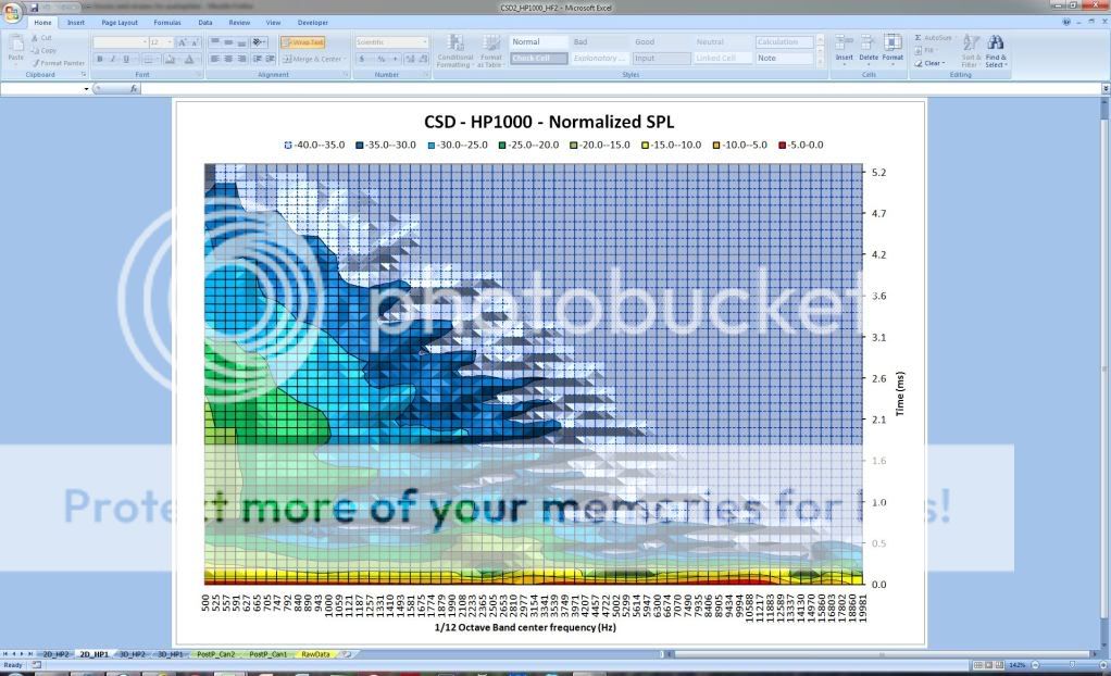
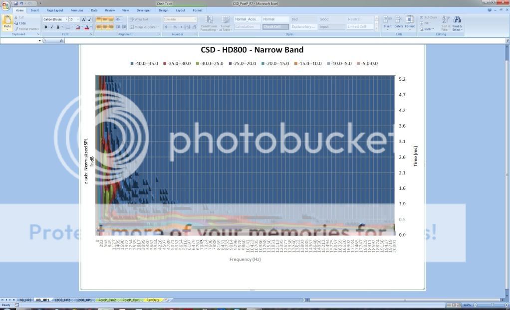
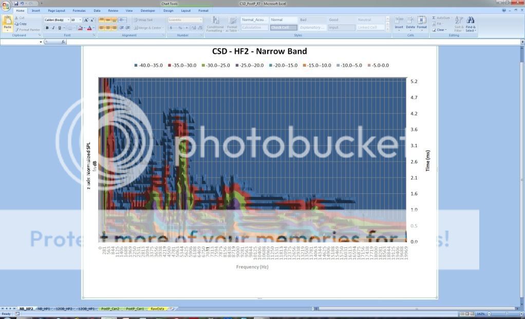
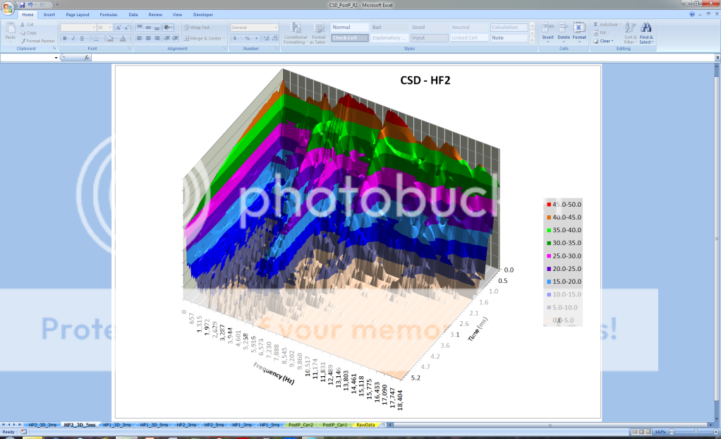
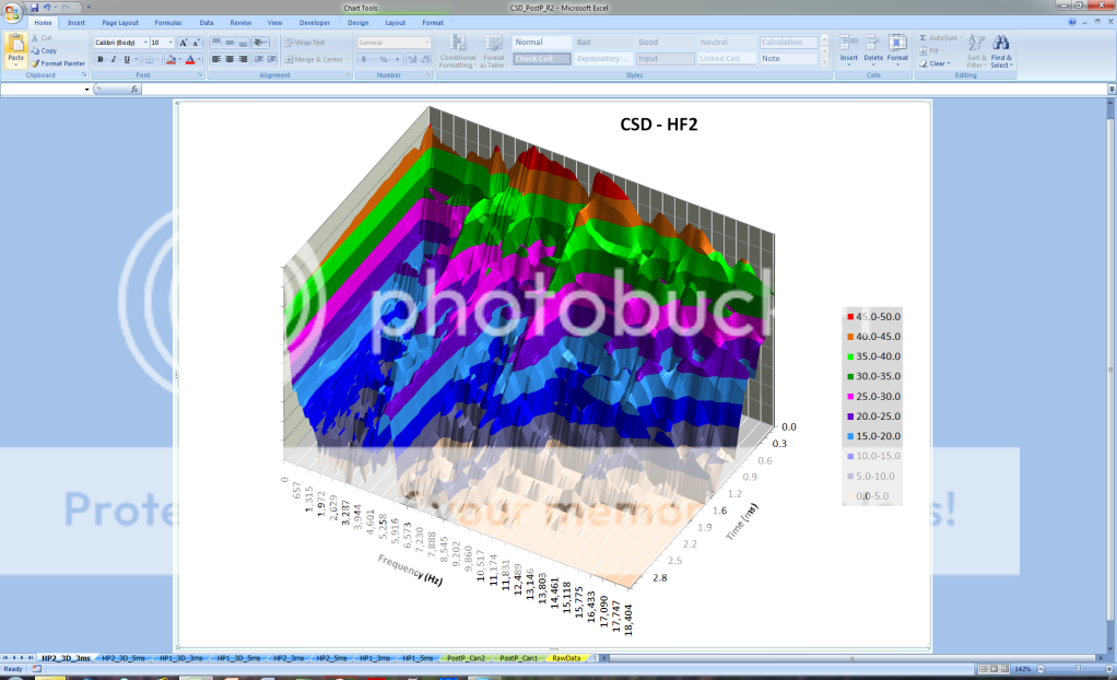
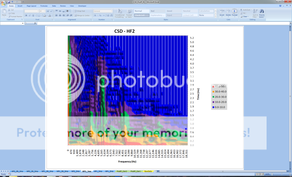
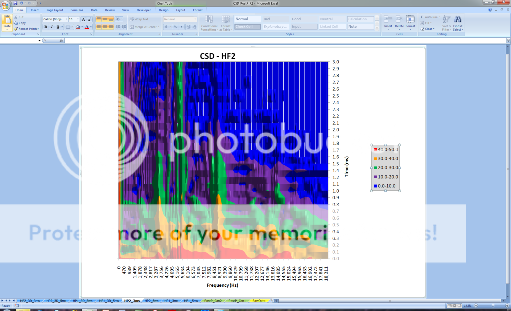
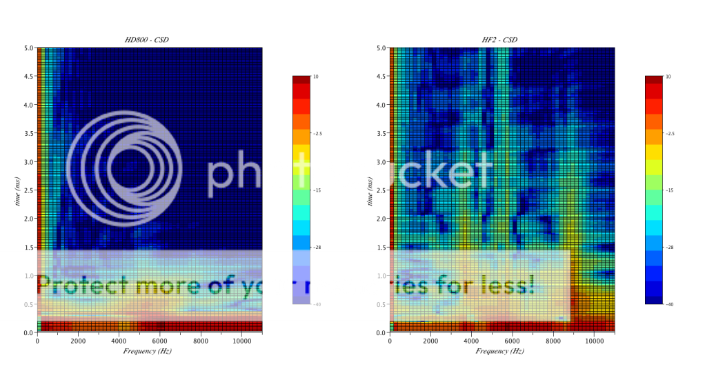
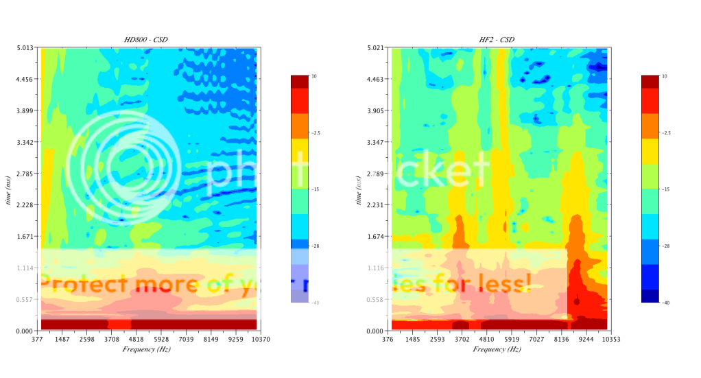
A new attempt at making the graphs more readable, still in Excel, the waterfall view shows normalized SPL (down to -40dB) in 1/12 Octave Bands. The 2D "top view" shows the narrow band results (also truncated below -40dB which is pretty much the usable range for this current data):

So Tyll, shall we proceed with your data ?

[Electrostatic Headphone Measurements]

cobra_kai, it's funny because I had the exact same thought process... When I failed to run Octave on either platforms, I looked into scypi since this actually might also become useful for my work. I spent a little bit of time looking at it (spyder on windows) and liked it enough (learning curve from Matlab is about 10x that of going to scilab though) to try to get similar tool for my mac at home. Turns out getting a nice interpreter like spider on the mac was way beyond my IT skills and I ended up forced to restore Lion from my backup . Then started the quest to dual boot Lion and Ubuntu, which went nowhere (MBP'11 not supported much, for example no wireless or trackpad so it was not really practical, plus I could never get it to boot anyway). Anyhow, I ended up installing Windows 7 and been actually very happy with that. The OS is almost as nice feeling as OSX and I can run python on it... In all, although I like to recommend macs for most anyone, I would say that in this particular case, it's been hell!!

TMoney: Stereophile's introduction to their standard speaker tests gives you some explanation about what it is and more importantly what it tells that a regular magnitude response function in 2D doesn't: http://www.stereophile.com/content/measuring-loudspeakers-part-two-page-5

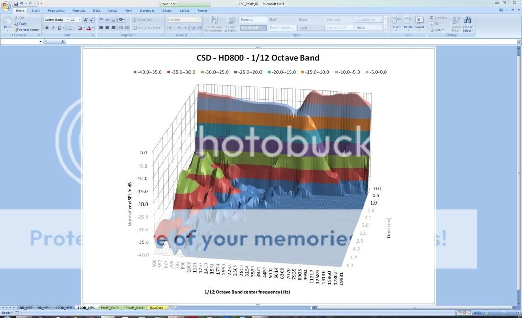
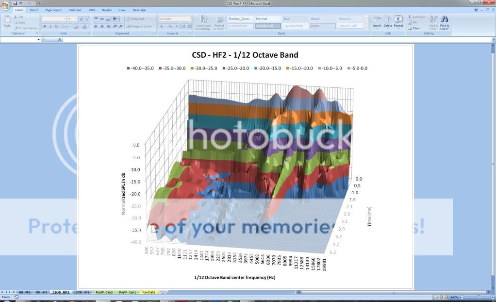
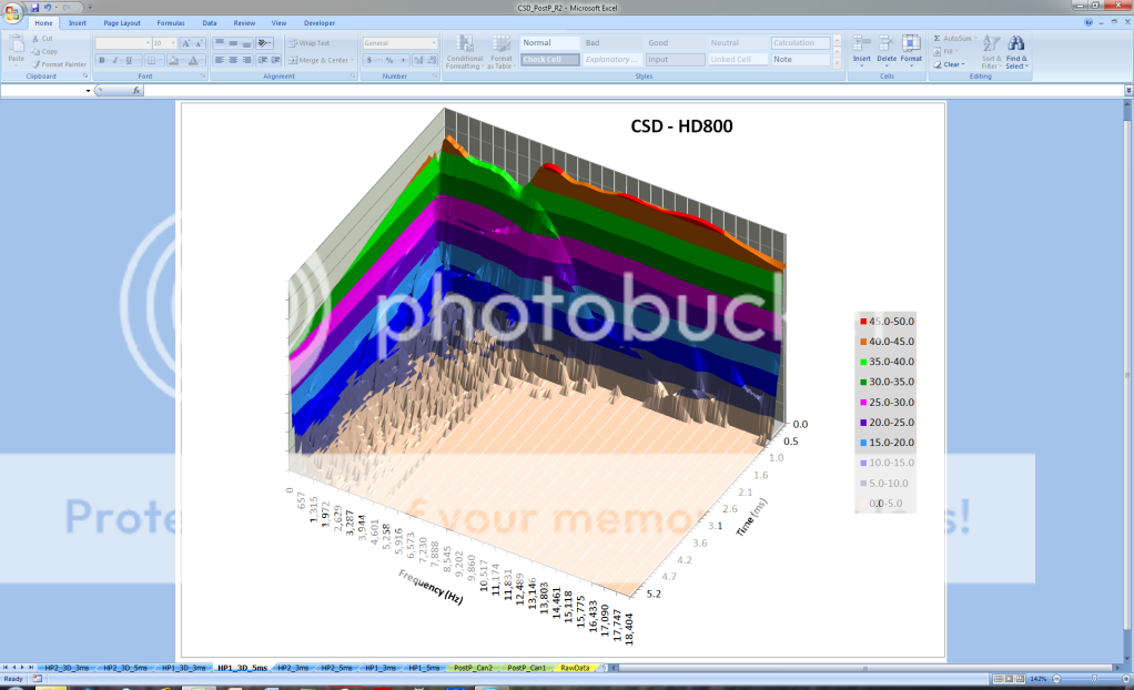
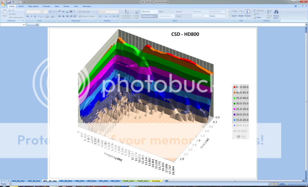
As cobra_kai said concisely, the extension into the 3rd direction is time. Think of it as the frequency response magnitude of the headphone, but only analysing the trailing edge of the impulse response. The first line (at t=0) is actually the exact same curve as published by Tyll up to now, it is the frequency response magnitude of the headphone using the whole data from rise of the impulse to its full decay a few ms later. The FRF slices down the time line truncate the beginning of the data so you're looking essentially at the ringing signature of the headphone. What you typically see is that peaks in the standard FRF magnitude curve ring for some time such that a ridge is formed at those frequencies.

In the case of the HD800 example, it is a bit hard to see as the headphone measures near perfect with just a tiny bit of ringing at 6kHz. In the case of the HF2, acoustic resonances of the undamped rear chamber for example (somewhere between 2 and 4kHz) clearly show up as they take several ms to decay by 40dB or so. As mentioned in the Stereophile introduction, you're pretty much guaranteed to hear those resonances in the midrange / lower treble so the graph is very useful to really gauge the behavior of the headphone. 2D magnitude curves typically make you miss that point in case the resonances are not clearly standing out.

Now, the issue at hand with headphone measurements is that you may not be able to look at such CSD graph with standard data which includes reflections from artificial (or not) pinna. In the case of speakers, measurement is performed in an anechoic room or in a standard room but truncating the impulse response before you see the first wall reflections (such as 6-10ms). In the case of headphones, Purrin's data looks really good but the man got some talent!

However, personally, I am not convinced yet that a standard headphone test on dummy cannot be used. The reason is that you are looking at some reflections no matter the test setup, if only the acoustic reflection from the back of the chamber to the ear. In the case of speaker, Stereophile rightfully mentions the test should be performed in anechoic conditions, but it is simply to remove the room dynamics (else you'll see the room modes decay, not that of the speaker). As discussed in the HF thread, at least with Purrin's data, the reflections from the room where the test was done are almost in the noise floor (50dB down) and don't prevent to look at the CSD of the headphone. Tyll is doing his tests in anechoic conditions (at least above 1kHz) so this should return even cleaner graphs.

sorry for the long rumbling post

[Electrostatic Headphone Measurements]

Neat work arnaud. In case anyone is interested, Octave is another free program that is similar to matlab, and will actually run many .m files that were written for matlab directly as long as it doesn't use stuff from fancy toolboxes.

Thanks, I did try to run Octave, both on OSX Lion and Win7, but no luck. I even tried installing Ubuntu on my mac to run it natively but never got that to run either... Scilab is sort of a more rigorous version of Matlab from the little I have played with it and as such, you systematically have to rewrite routines. I ended spending quite a bit of time on Scilab but kind of like it now. Graphs are actually cleaner than Matlab.

[Electrostatic Headphone Measurements]

Tyll, no worries... You probably also got skeptical when you saw the SPL scale ;o). That's corrected now, I had forgotten to divide the fft by delta_t... In regards to integrating this into your existing spreadsheet, it's probably not recommended because of the large size of the CSD results (probably +1.5MB for each headphone Excel file). Also, you should try it with a couple of your data first as there's a possibility a "standard" dummy head measurement does not accommodate well with this (ask Purrin about his brilliant idea, I cant reveal it for him ;o) ).

Still, if you wanted to process your existing data again with that additional result, I am pretty sure we could come up with a macro to automate the loading of data for these 100+ files... Let me know, I'll be glad to help,

arnaud

[Electrostatic Headphone Measurements]

Thanks Torpedo,

I actually updated the file, it now runs up to 5ms which helps with the HF2 sample data. As for Excel macro itself, it's really no big deal, you just press record and see what it did, then copy that over . In retrospect, although this is not as flexible as a proper tool like Scilab, it's clearly a better approach to share around as most anyone can use and possesses Excel.

arnaud

[Electrostatic Headphone Measurements]

Tyll,

The Excel post-processing did not turn out too bad! I made a macro to automate the fft calculation of 50 time slices (zeroing the first time steps, by pack of 5 at every step). Much more could be done to give more flexibility (such as the resolution in the time axis), but for now here is how it's setup:

• I am using Purrin's data, which is 48kHz sample rate
  
• The macro does an fft on the first 512 data steps, which is about 10ms of data (512/48000)
  
• The frequency resolution is about 100Hz (48000/512)
  
• The ffts are repeated with truncated data by blocks of 5 steps, so basically you see the FFT at 0 0.1 0.2 0.3ms and so on
  
• 50 ffts total are computed to you get the decay curve up to about 5ms
  
• Time decay graphs are generated for the 2 headphones data
  
• Time decay graphs are presented in 2D and 3D, I find the 2D version more readable though
  
• For each graph type, there are 2 versions, one that cuts at 3ms, the other at 5ms
  
  
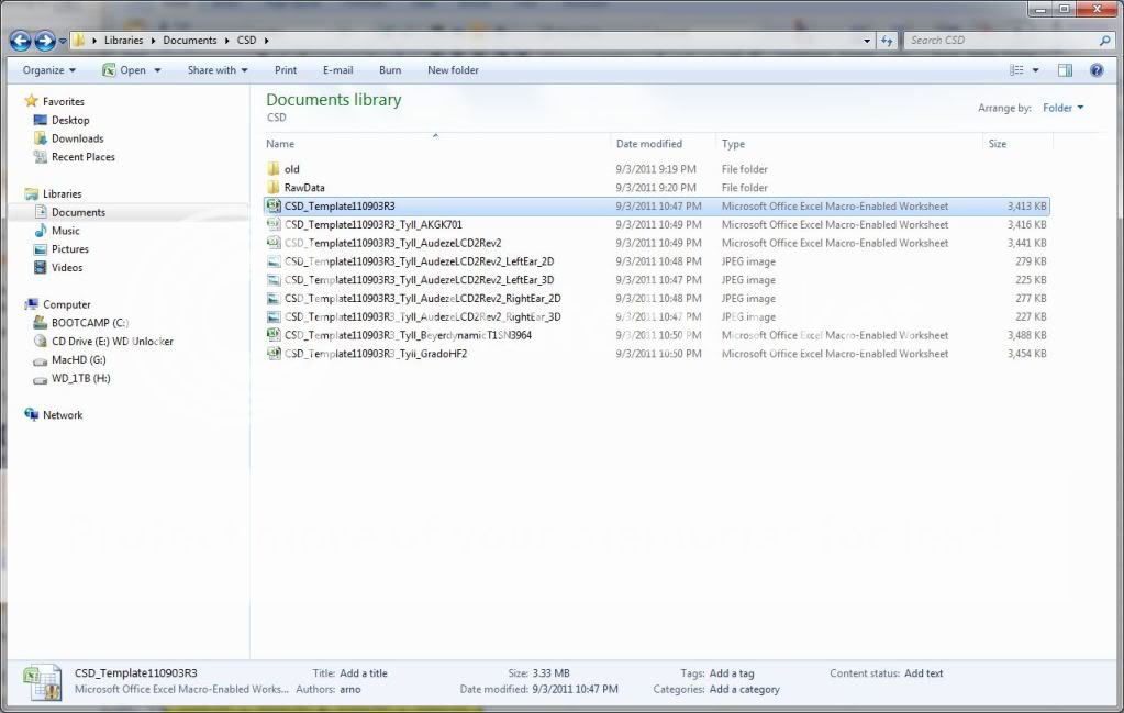
  In order to use the Excel file:
  • You need to enable the analysis toolpack (an add-on) as well as macros
    
  • In the RawData tab, you paste your data in the yellow zone
    
  • In the same tab, you click first on step 1 button, then click on step 2 button
    
  • You then have the CSD graphs updated in their own tab
    

  Here are some screen shots:

  

  

  

  

  

  

  

  

  

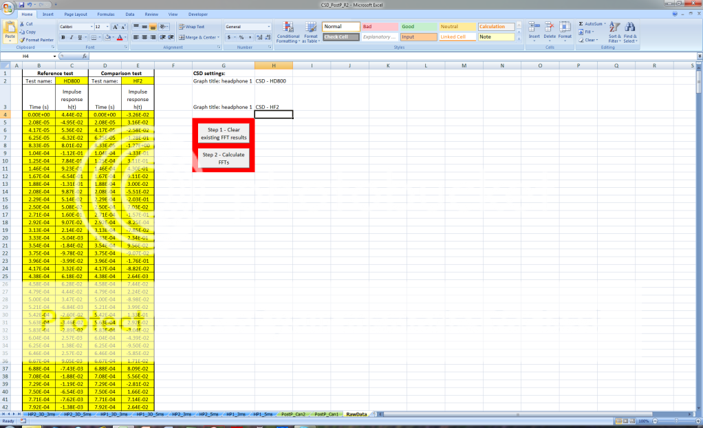
  PM me with your email if you want the Excel file (under 3.5MB),

  cheers,

  arnaud

[Electrostatic Headphone Measurements]

Hi Tyll,

As Purrin said, it's all in the impulse response. Frankly speaking, I hadn't thought of using Excel, which might be the most convenient way to share the post-processing routine with you. I will have a look at it later on. I believe the fft in excel is limited to 4096 taps but that should be sufficient for headphone measurement data on a dummy head).

Meanwhile, I have actually rewritten my routine on Scilab, which is very to similar to the pricey Matlab code, but free. It's pretty stable (except on OSX Lion), runs on several platforms: http://www.scilab.org/

Since I did not create any GUI for the script, you'd need to edit the first few lines (see screen shot below) to:

> Line 5: change the path where the files are located

> Line 21: provide the measurement file name for the "reference headphone" (currently a 3 column Excel file with time, real, imaginary part of the impulse response)

> Line 22: type the reference headphone name

> Line 23: enter -1 if you want the impulse response to be inversed (the data I got from Purrin needed it for the SR80 and HF2)

> Line 24: enter the oversampling rate (can be 1, I use 2 to make the CSD data look a bit smoother)

> Line 25: enter the number of "slices" for the waterfall graph (1 slice is = 1/Fsamp (sample rate of data acquisition). I need only 70 steps (48kHz measurement rate) to see the HD800 decay to -50dB, Grado's recent headphone need a bit more

> Repeat from line 38 to 42 for the "other headphone"

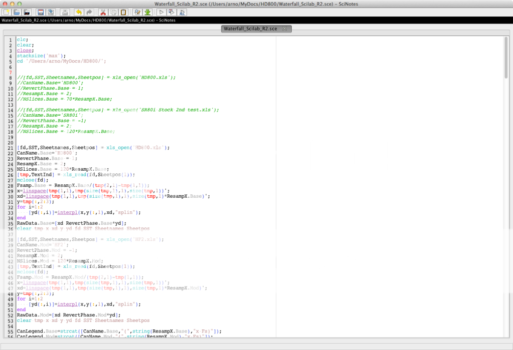
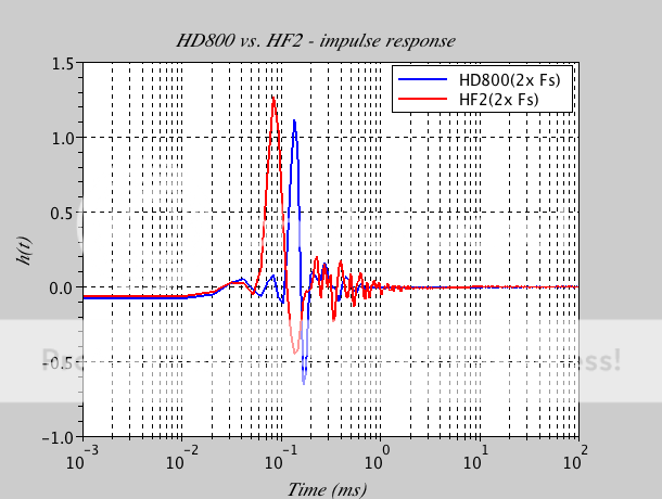
Here are example shots of the routine, comparing HD800 stock form to HF2 headphones (figures are automatically saved to the folder where the script and data resides):

The standard results you're already generating:

The waterfall plots (can display it in 3D view but it's much more readable from top view):

I think I can do something similar with Excel but might not look as clean. Will give it a shot and let you know!

[Electrostatic Headphone Measurements]

Hi Tyll,

I sent you an email at inner fidelity adress in regards to waterfall plots, any plan to include that in the standard tests? Purrin posted some example in the sr009 thread and it's quite useful at revealing resonances. In case you don't have the tools to post-process it, I wouldn't mind generating the graphs for you from the impulse response data...

Otherwise, I could mail you my 009 but I am a bit concerned with damage during transport, esp. since we never got confirmation that the troubles with previous batch were not related to transport...

[The Headcase Stax thread]

Assuming somebody knows something just based on their education isn't a very good way to go. Take my EE Phd. cousin who had no idea how a dynamic speaker worked...

This is hilarious! To be fair though, the deeper you go in a given field the more focused you get and the more you loose ground on reality... That doesn't mean you should forget the basis though .

On a similar level, I've met bright technicians and terrible PhD (not meaning your cousin does not earn his PhD ... unless he's the same person who confused the K-1000 with an ES can over at HF in the sr-009 thread from Jude, lol )